Introduction to Pix4D Software

Developed by Pix4D SA as a web-based standalone product for Microsoft Windows, Pix4D is one of the current premier software for photogrammetry. It’s many applications include creating professional orthomosaics, constructing point clouds, generating models and more. With it’s simple layout and automated tools, it is incredibly easy to use. The proper background knowledge is necessary to understand the information that is being generated and to ensure that the tools are used correctly and the results interpreted ethically.

Photogrammetry is the technique to extract geometric information from two-dimensional images or video. For a comparison of photogrammetry software, click here. 

This post contains:

• A basic introduction to the Pix4D software
• A brief tutorial for performing basic functions in Pix4D Mapper
• A final overview of the software with links on where to find more information

Introduction to Pix4D

Figure 1 The illustrated workflow of Pix4D software.  Source: Pix4D User Manual

• CAPTURE: The user can capture an image with any digital camera or use Pix4Dcapture flight planning app on your mobile or tablet for drone field operations, flight review, and optimal data capture.
• PROCESS: Choose offline processing on Pix4D desktop for full control over data, without needing an internet connection. Choose online processing for fully automated, hardware free results on Pix4D cloud.
• ANALYZE: On desktop, gain access to advanced editing features, quality control, and measurements. For the cloud, monitor projects over time, use the drawing overlay for construction, and automatic NDVI map for agriculture.
• SHARE: Easily collaborate and annotate projects online, then share maps, models, and analytics with a simple URL.

Data Acquisition

The images that form the dataset must be obtained in the field before using Pix4Dmapper. It is recommended to use images that have geolocation and Ground Control Points (GCPs) for more accurate results.

In order to take a good dataset, there are four steps:

1. Design an Image Acquisition Plan: Considering key details ahead of time will mitigate problems and ensure that data collection is as thorough and efficient as possible. Is the project aerial, terrestrial, or mixed? What type of terrain or object will be photographed? What type of camera will be used? At what rate will the images be taken? What is the ideal flight height and angle? Draw out a path for ideal image collection. For aerial projects, this includes selecting the corridor path or regular and/or circular grid. Always keep the purpose of the project in mind.   

2. Configure the camera settings: Wrong configuration can result in images with blur, noise, distortions, etc. There are specific requirements necessary to collect agricultural data, etc. so the specific project type should be researched ahead of time to avoid any problems.  

3. Georeference the images: While this step is considered optional, it is highly recommended to avoid data mishaps later. The images can be georeferenced using a camera with built-in GPS or by external GPS devices. 

4. Getting Ground Control Points (GCPs) on the field or through other sources: Again, though optional, this step is recommended to ensure data accuracy. Plan how many GCPs have to be acquired and include their measurement in the Data Acquisition Plan.

What are the recommended hardware and software requirements?

Windows 7, 8, 10 64 bits is recommended, as is a CPU quad-core or hexa-core Intel i7/Xeon. Your computer should be GeForce GPU compatible with OpenGL 3.2 and 2 GB RAM. Solid-state hard-drives are best.

• Small projects (under 100 images at 14 MP): 8 GB RAM, 15 GB SSD Free Space.
• Medium projects (between 100 and 500 images at 14 MP): 16GB RAM, 30 GB SSD Free Space.
• Large projects (over 500 images at 14 MP): 32 GB RAM, 60 GB SSD Free Space.
• Very Large projects (over 2000 images at 14 MP): 32 GB RAM, 120 GB SSD Free Space.

What is the overlap needed for Pix4D to process imagery?

At least 75% frontal overlap is required for most cases and at least 60% side overlap, though the desire percentage changes depending in the terrain type. This detail requires careful planning. The image acquisition plan depends on the required Ground Sampling Distance (GSD) in the project specifications. The GSD will define the flight height at which the images have to be taken. This is heavily dependent on the project specifications and the terrain type or object to be reconstructed.

Nowadays, advanced Unmanned Aerial Vehicles (UAVs) come with very good software that can design the image acquisition plan automatically when given some parameters. These smart little robots can automatically take the required images according to the selected acquisition plan with no need for the user to intervene.

What if the user is flying over sand, snow, or uniform fields?

The generally recommended flight path can be seen in Figure 2. Modifications on this path can be made for different types of terrain. For example, flat terrain with homogeneous visual content such as agriculture fields requires a frontal overlap of at least 85% between images and at least 70% side overlap. For this type of terrain, flying higher improves the results. Having accurate image geolocation is necessary and use of the Agriculture template is recommended (click here for more details).

For snow and sand, at least 85% frontal overlap and 70% side overlap is again recommended. To avoid washout, it is important to set the exposure settings to get as much contrast as possible.

For water surfaces (including oceans, lakes, rivers, and ponds), sun reflection and lack of visual content to aid in point matching are problematic. Pix4D cannot reconstruct water bodies as large as the oceans, but to reconstruct other water surfaces, each image needs to include land features. Flying higher may help.

Figure 2 This graphic demonstrates the flight path. over the area of interest. Each red circle represents an image that was taken during the flight. Overlap is necessary to piece the images together into a cohesive map of the area.

What is Rapid Check?

Rapid Check is a program that runs inside of Pix4D and is used as an alternative initial processing system where accuracy is traded for speed. It processes quickly in an effort to determine whether sufficient coverage was obtained, but the result has fairly low accuracy. The rapid check is for field use to verify whether the proper areas and coverage of data were attained.

Can Pix4D process multiple flights?

Yes, Pix4Dmapper can process images taken from multiple flights provided that four factors are accounted for:

1. The same flight height is maintained
2. Each plan captures the images with enough overlap
3. The image acquisition plans overlap one another adequately (Fig.3)(Fig.4)
4. The flights are taken under very similar conditions (sun direction, weather conditions, no new buildings, etc.)

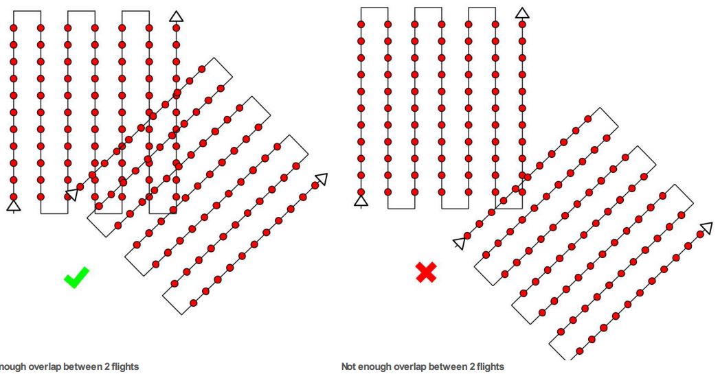
Figure 3 In order for Pix4D to process data from multiple flights, the flight path must overlap at least as much as the diagram on the left. Source: Pix4D 3.0 user manual.

Figure 4 The recommended image acquisition plan overlap for multiple flights.

Can Pix4D process oblique images?

Yes. Oblique imagery (Fig.5) is recommended for use in building reconstruction and other 3D objects.  This requires a specific image acquisition plan which includes flying around the object a first time at a 45° camera angle, followed by a second and third time around the building increasing the flight height and decreasing the camera angle with each round (Fig.6). Taking one image every 5-10 degrees is recommended to ensure enough overlap, depending on the size of the object and distance to it. Shorter distance and larger objects require images every less degrees.

Figure 5 Oblique imagery gives the viewer a reference to the height of an object. Source: Pix4D User manual.

Figure 6 An example of the ideal image acquisition plan for a 3D object, such as a barn. Source: Pix4D user manual.

Are GCPs necessary for Pix4D? When are they highly recommended?

While ground control points (points of known coordinates in the area of interest) are not necessary for processing in Pix4D, they are highly recommended in certain cases:

• Corridor mapping with a single track (which is to be used ONLY when a dual track image acquisition plan is not possible). This requires at least 85% frontal overlap and GCPs that are defined along the flight line in a zig zag formation.
• Images without geolocation.  When images have no geolocation, Pix4Dmapper can use GCPs to locate, scale and orient the model. 
• When particularly high accuracy is needed.

What is the quality report?

The quality report is automatically generated for each project in Pix4D and can be opened by clicking Process>Quality Report on the main tab bar. This opens a report that can be downloaded and saved as a pdf (Fig.7). 

Figure 7 The quality report pdf is generated automatically. 

This report contains a summary of all aspects of the project, including: a preview (Fig.8), initial image positions, computed image/GCPs/Manual Tie Points Positions, GCPs/Check Points, absolute camera position and orientation uncertainties, overlap, internal camera parameters (including perspective lens and fisheye lens), 2D Keypoints Table and 2D Keypoint Matches graph, relative camera position and orientation uncertainties, 2D Keypoint Table for Camera, a table showing Median / 75% / Maximal Number of Matches Between Camera Models, 3D points from 2D Keypoint Matches, Manual Tie Points, Ground Control Points, scale constraints, orientation constraints, absolute geolocation variance, geolocation coordinate system transformation, relative geolocation variance, and rolling shutter statistics.

Figure 8 This image, taken from a quality report generated for the Litchfield Mine in Eau Claire, Wisconsin, shows the typical low resolution preview of the Orthomosaic and the DSM (digital surface model). They allow a visual inspection of the quality of the initial calibration.

To see an online example of a quality report, click here.

For more information on quality reports, click here to see the Pix4D support page. 

A Tour of Basic Functions

Processing Data

Open Pix4Dmapper and click Project>New Project. Choose a folder to save to. Select Add images and open the data files. In this example, the data are aerial images taken by Dr. Joseph Hupy  of UW Eau Claire using a DJI Phantom UAV. The study area is the Litchfield Mine, adjacent to the Chippewa River in Eau Claire, Eau Claire County, Wisconsin. The WGS 1984 UTM Zone 15N coordinates system is detected automatically by Pix4D. Upon opening a new project in Pix4D, the user is prompted with an option then to expand the project. For today’s purposes, a simple project (the default settings) will do (Fig.9). Click finish. 

Figure 9 This menu displays options to expand the report. The basic, preselected options include a 3D model, an orthomosaic, a DSM, a 3D Mesh, and a Point Cloud. Using this information the user can measure volumes of objects, digitize objects, generate contour lines, and more.

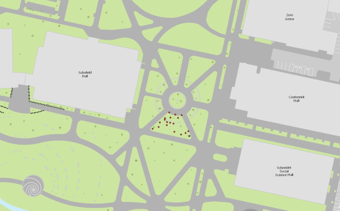
The flight pattern is shown via points and lines over a basemap of the area (Fig.10).

Figure 10

Analysis of the quality report

After the initial processing is done, examine the quality report.

The following steps are recommended:

Quality Check. Verify that: all the checks are green, all or almost all the images are calibrated in one block, the relative difference between initial and optimized internal camera parameters is below 5%, and, if using GCPs, that the GCP error is below 3×GSD (Fig.11).

Figure 11 In the Litchfield Mine project report, the Quality Check revealed that all 68 images were calibrated (meaning that none were rejected for not overlapping enough) and Pix4D was able to automatically generate 8553.1 matches between images in order to overlay them accurately.

A red flag was raised by the Camera Optimization. This indicates that the focal length/affine transformation parameters, which are a property of the camera's sensor and optics which varies with temperature, shocks, altitude, and time, was not within 5% of the optimized value to ensure a fast and robust optimization.

The Georeferencing raised a yellow flag because no 3D ground control points were used, which means there may be a decrease in accuracy of the 3D model.

Examine the Preview. For projects with nadir images and for which the orthomosaic preview has been generated, verify that the orthomosaic does not contain holes or have distortions. If GCPs or image geolocation has been used, make sure that it has the correct orientation (Fig.12).

Figure 12 In the preview generated for the example project (right) compared to the aerial image of the Litchfield Mine (left), there are no holes in the data. Few distortions are apparent, though there appears to be an area of poor overlap in the center, indicated in this image by the orange rectangle. This may be because fewer photos were taken over the northern portion of the mine because there is less relief there.

Calculating surface area within the rayCloud editor

The use of the rayCloud is optional and it can be used to:

• Visualize the different elements of the reconstruction and their properties.
• Verify/ improve the accuracy of the reconstruction of the model.
• Visualize point clouds / triangle meshes created in other projects or with other software.
• Georeference a project using GCPs and /or Scale and Orientation constraints.
• Create Orthoplanes to obtain mosaics of any selected plane.
• Assign points of the point cloud to different point groups.
• Improve the visual aspect.
• Create objects and measure distances (polylines) and surfaces.
• Create 3D fly-through animations (Video Animation Trajectories).
• Export different elements, such as: GCPs, Manual / Automatic Tie Points, Objects, Video Animation Trajectories.
• Export point cloud files using points belonging to one or several classes.

In order to calculate surface area of on object, such as a sand pile, click View>rayCloud on the Menu bar (Fig.13). Note: If the image does not resemble the figure below, then follow the steps above to process the data, then open the rayCloud.

Figure 13 The rayCloud view indicated the area of each image that was taken along the flight path and the angle each is associated relative to the ground.

In the left sidebar, click rayCloud>Surface (Fig.14). The measurements will be displayed in the right sidebar. 

Figure 14 The surface box must be selected to view measurements such as projected 2D length and enclosed 3D area. 

Calculate the volume of a 3D object

In order to create a new volume, click View>Volumes>New Volume on the Menu bar. On the 3D View, a green point appears beside the mouse. Left clicking the feature will mark the vertices of the base surface of the volume. With each click a vertex is created and the volume base surface is formed. Right clicking indicates that the feature is encircled and creates the volume base. On the sidebar, click Compute to compute the volume (Fig.15). For further instruction on this, click here. 

Figure 15 This compilation of images shows the sequence of steps to compute the volume of an object in Pix4D. The calculations are displayed in image 4. 

How to export a volume

On the Menu bar, click View > Volumes. On the sidebar, in the Objects section, click the symbol that resembles a square with an outward-facing arrow. Click All to select all Volumes to be exported, click None to unselect all Volumes or select the checkbox on the left of each Volume to select some of the Volumes to be exported (Fig16). Click export and save the image as a .shp file in order to open it in ArcMap (Fig.17). The metadata will need to be added manually.

Figure 16 The export symbol is indicated by the arrow.

Figure 17 The shape files can be imported in Arcmap for map making.

Overview

This concludes the brief overview of a few of the basic functions that can be performed using Pix4D software. 

Further information can be found at: 

Pix4D website 

Offline Getting Started and Manual  

Extended Software Manual

Articles on how to use the rayCloud

Field Activity #8: Survey of point features with a dual frequency GPS

Introduction

This assignment served as an introduction to surveying with high precision GPS unit. The class collected elevation data of a very small defined area as a group and then created continuous surface raster layers using the five common interpolation methods: IDW, Kriging, Natural Neighbor, Spline, TIN. 

Study Area

The area of study was a small grassy knoll in the heart of the UW Eau Claire campus mall. This area between Centennial, Schofield, and Schneider Halls is affectionately known as the “black tombstone ring,” so called because of the black stone benches which are arranged in a circle around the iconic Sprite statue (Fig.1). Our knoll is at the base of the sprite statue on the side closest to the science building, Philips Hall.

Figure 1 The Sprites statue is at the heart of the campus mall of  UW Eau Claire. Upon completion of Centennial Hall in 2015, the Sprites statue was moved to this pedestal surrounded by black stone benches and symmetrical knolls. Photo credit: Jim Arnold. 

The knoll forms the shape of a small trapezoid, little more than 20 square meters bounded on four sides by sidewalks (Fig.2). It contains five tiny ornamental saplings and four black stone benches, which are very abstract and artsy looking, though in a decidedly more simplistic vein than the Sprite statue. The elevation of the knoll is defined by a small hillock running along the wider southern face of the knoll. The four stone benches are on a flat area facing the Sprite statue.  

Figure 2 The study area is denoted by the arrow. This image is from Google Earth Pro (2016). The Sprite statue is in the center of the ring. 

Materials

• Survey grade GPS: TopCon HiPer SR
• TopCon Tesla handheld unit
• ArcMap for Desktop 10.4.1

The TopCon equipment (Fig.3) made data collection very simple and efficient. The HiPer SR was mounted onto a survey tripod that had a level to ensure that the GPS unit was parallel to the ground. The Tesla handheld unit was used to enter the data.

Figure 3 The TopCon Tesla handheld unit and the TopCon HiPer SR, the high precision GPS unit which can record elevation and location to sub-centimeter accuracy. 

Methods

The class walked to the study area and received an instructional demo from Dr. Hupy about how to position the tripod and GPS unit, and how to record data using the Tesla handheld unit. Each person in the class took a turn positioning the tripod and recording 1-3 data points within the small grassy knoll (Fig.4). The class, after discussing sampling methods, went with a simple stratified point collection method because of its flexibility. Special attention could be paid to the edges of the hill and in defining the extent of the flat area.

For more information on sampling methods, check out the Royal Geographical Society page. 

Figure 4 This figure shows the UWEC campus and the study area with the collected data points.

The result was a data table of nineteen points of elevation data which was shared to the class as a txt file which was located in the TEMP folder. This had to be copied into individual student folders and normalized. The data was downloaded into Excel using the Data>From TXT command. Normalized the formatting by changing headers to Point_ID, Y, X, and Z (Fig.5).

Figure 5 The normalized data ready to be imported to ArcMap!

In ArcMap for Desktop, a file geodatabase was created and the excel table opened. Selecting the “Display XY Data” option created an event theme. The coordinate system was set to NAD 1983 UTM Zone 15N. Then the event theme could be exported as a point feature class.

In order to transform the point data into continuous surface rasters, interpolation tools were necessary to mathematically generate elevation values to fit between the collected data points. (See the Activity #5 post for information on interpolation techniques.) The five common interpolation methods -- IDW, Kriging, Natural Neighbor, Spline, and TIN—were run on the data using the respective tools. In order to define the study area, a polygon feature was created to show the boundary of the study area and then used as a mask to clip the interpolation results. Unfortunately, there was no tool to clip the TIN results.

Results/Discussion

The elevation results were less than dazzling. The actual shape of the hill was not captured accurately in any of the continuous surface results (Fig.6). It is clear that there were sampling problems with the data, the most obvious problem being the small sample size of elevation points collected with the GPS.

Figure 6 The results from the various interpolation methods compared to an aerial image of the study area from Google Earth Pro (2016). The orange points indicate the data points collected by the class. Notice that there are areas where no data was collected; this had a negative impact on the accuracy of the interpolations.

Sampling problems are a part of map making that is common and dangerous. According to the Royal Geographical Society, these are some of the considerations one must make when sampling a study area:

• Larger sample sizes are more accurate representations of the whole
• A sampling strategy made with the minimum of bias is the most statistically valid
• Most approaches assume that the parent population has a normal distribution where most items or individuals clustered close to the mean, with few extremes
• Sampling, no matter how good can only ever be claimed to be a very close estimate

Regarding the stratified sampling method that was used in this field activity, the proportions of the sub-sets must be known and accurate if it is to work properly. Not only did the class not measure and record the proportions of sub-sets, there were no sub-sets set up in the first place. In the ArcCollector Activity done in November, the class also used a stratified sampling technique when collecting data points around the UWEC campus, but the campus was split into five distinct zones to ensure somewhat even coverage of all areas. In this activity, however, the data collection was unorganized and uncoordinated, and that clearly had a negative impact on overall accuracy.

In this assignment, there were only 19 data points to work with, which was not a large enough sample size to interpolate the elevation of the area accurately. Since the area was so small, the class easily could have collected more points. However, being limited to one GPS unit meant there was quite a bit of standing idle and the cold rain was good motivation for the students to cut the data collection short.  

Conclusions

Overall, the final product suffered from a lack of data. None of the interpolated elevation maps captured the true relief of the study area. This activity served as an excellent intro to TopCon products and data collection with survey grade GPS units, but did not result in accurate maps of the study area. 

UWEC campus mall. Photo Credit: Bill Hoepner

Arc Collector Activity 2: Putnam Prairie Research Project

Introduction

In the previous lab, the class used Arc Collector to add data to an online database that was created beforehand. For this project, each student needed to create their own infrastructure to collect data about a topic of their choice. The objectives were to think of a geospatial research question to design a project around, create a database with three or more feature classes that would implement the research objective and deploy it to Arc Collector, collect point features, and then write a report to explain the results. The report, of course, had to include maps and use the data to either support or refute the research question.
As a conservation biologist, it was natural to gravitate toward a biology research topic. Two semesters ago in the fall of 2015, the Conservation Biology 328 class implemented an invasive species removal plan in the Putnam Prairie area.  The project focused primarily on the mechanical removal and chemical treatment of invasive Black Locust trees (Robinia pseudoacacia). This invasive tree is prolific in the area and provides many management challenges, and there was some trepidation as to whether the removal strategies would help or just aggravate the problem.

This seemed a perfect opportunity to answer the question once and for all: Did the black locust removal attempt succeed in removing black locust from Putnam Prairie or did the control attempts worsen the problem?  

Some smaller questions to address:

·         Has black locust returned in the areas where we removed it?

·         Was the removal treatment effective in killing the treated stems?

Materials:

·         Nexus 9 Android tablet borrowed from the Geography department. (It has a built in GPS, unlike an iPad)

·         Arc Collector

Black Locust (Robinia pseudoacacia)

Black locust is a fast growing deciduous tree which is commonly 30-80 feet tall. Native to the Appalachian Mountains throughout Pennsylvania to Alabama, it has spread throughout most of the contiguous United States as an invasive species. Movement to new areas was often facilitated naively by landscapers, who valued the species for its aesthetics and rot-resistant wood. It thrives in disturbed habitats with full sunlight, such as prairies or floodplain forests. It grows best on well-drained soil with sparse competition.
It has pinnately compound leaves and highly fragrant white flowers which give way to hanging seed pods. Trees and saplings feature prominent woody spines along the trunk and branches, which makes it easy to identify a black locust even in the winter (Fig.1).

Figure 1 Identifiable characteristics of the species Robinia pseudoacacia. The prominent woody spines made identification simple, since there were no leaves, pods, or flowers at the time of data collection. 

Table taken from "A Weed Report" from the book Weed Control in Natural Areas in the Western United States, available through the UC Weed Research and Information Center.  

The tree produces numerous suckers from the roots and thus is capable of forming dense clonal colonies that exclude native vegetation. Root suckers, which form primarily where branch roots emerge from older roots, become new saplings very quickly when the main stem of the black locust is disturbed. This is known as vegetative regeneration and in black locust it is considered a more common means of reproduction than seed. Sprouting often occurs in response to stem or root damage due to cutting, fire, wind, or disease. This creates a huge challenge for the control of black locust, since areas of abundant sunlight allow for one tree to become a dense thicket of trees when any form of removal is attempted. (For more information on vegetative regeneration, click here!) 

Typically, the root system of an established black locust tree has a radial extent of 1 to 1.5 times tree height. Root extensions of 165 feet were documented in the Appalachians. In the sandy soil of Putnam Prairie, extensive lateral root systems are to be expected. (For more information on this, click here!)

Area of Interest

Putnam Prairie is a small area of land near the main UW Eau Claire campus (Fig.2). It is considered a “postage stamp prairie”, an area that has been a prairie since before the city of Eau Claire was built around it. Unfortunately, Putnam Prairie is being inundated with multiple invasive species, including burgeoning thickets of black locust, which are excluding the native grasses.

Figure 2 The Putnam Prairie is attached to upper Putnam Park, adjacent to the UW Eau Claire campus and Sacred Heart Hospital. 

Figure 3 These two images show a comparison between the Putnam Priaire in fall of 2015 and summer of 2016. The left image is from the ESRI basemap (TerraColor satellite imagery, NAIP2015 Source: USDA FSA) and shows “leaf off” conditions. The black locusts are more difficult to spot without summer foliage, but the 2016 photo (Source: Google Earth Pro) shows the extent of the invasion. With the exception of three jack pines, all of the trees within the blue boundary are invasive black locusts.

The Fall 2015 Conservation Biology 328 class, under the instruction of UW Eau Claire Biology Professor Dr. Paula Kleintjes-Neff, completed a project early in December 2015 that centered around removal of black locust trees from Putnam Prairie. (The class report on this project can be viewed here.) Two physical control methods were used:  total removal by either by hand saw, or girdling using hand saws or serrated knives. All the removed or girdled trees were then treated using a mixture of the chemical herbicide triclopyr and mineral oil. This herbicide, advertised under names including Garlon or Crossbow, is selective in managing woody plants as well as herbaceous weeds.  When mixed with mineral oil, triclopyr is less toxic to native wildlife, and due to the selective nature of this chemical, native grasses are minimally affected by it. The class was informed that the most successful method for application is to cut the tree down and saturate the remaining base with this mixture (Fig.4).

Figure 4 An actual photo from the black locust removal performed by the students of Conservation Biology 328 in December 2015. The triclopyr herbicide was applied using spray bottles and applied liberally to the stumps or girdled area. Photo credit: Alexandra Johnson. 

The Fall 2015 Conservation Biology class was not the most recent class to implement invasive species removal in the Putnam Prairie. According to Dr. Kleintjes-Neff, the Spring 2016 Biology 328 class also cut, girdled, and treated black locust trees. According to Dr. Kleitjes-Neff, many of the trees treated December 2015 had new shoots regenerating from the stumps or and they were treated again by the Spring class, as well as many small trees that had not been treated previously. The future spring section of Biology 328 (Spring 2017) is also forecasted to participate in the removal.  

Methods

Step 1: Prepare the data in ArcGIS for Desktop

The ESRI online tutorial provided simple guidelines. 

1. A geodatabase called “Putnam_Prairie” was set up in ArcCatalogue.
2. Next, geodatabase domains were defined. This provided a list of choices the data collector can choose from while working, and cuts down on data entry error. For this project, data needs to be collected about tree height, whether the tree has been treated for removal, type of removal attempt (girdling/herbicide, hand saw and herbicide), and whether the tree is alive or dead.  Out of trees that are alive, are the roots regenerating shoots or not.
3. To define the feature class: “Black_Locust”, a point feature class, was added to the geodatabase. Coordinate system as WGS 1984 Web Mercator (auxiliary sphere).
4. Set up the fields. This is a key part of the information model. Fields provide the structure of the information collected in the field and provide rules for the types of information collected about a feature.

o   Tree_height: height of target plant (feet)

§  Range: 0-40 feet

o   Treated: Was the tree treated for removal last year?

§  Yes or No

o   Removal_type: What method of removal was attempted?

§  Girdling (A ring was cut around the trunk and then the stripped area was sprayed with herbicide) or Saw (Trunk removed by saw, stump treated with herbicide)

o   Status:

§  Alive or Dead

o   Regenerating: New shoots forming?

§  Yes (New shoots from stump or base of trunk) or No (No evidence of new shoots)

5. Theme the data: The symbology was set to green circles to keep the map simple.

6. Publish the data: The map was deployed to ArcGIS Online for mobile offline data collection.

Step 2: Data Collection 

Data was recorded over two days in mid-November by Amanda Senger using the Android tablet. The weather was just above 50 degrees F and windy. Attributes and photos were recorded for 197 black locust trees. The study area consisted of two main thickets of black locust with trees ranging from 2 to 7 feet tall (Fig.5). The three most common tree types to find were small untreated saplings, treated stumps that were sprouting new shoots, and girdled trees that were surrounded by young clones (Fig.6). 

Figure 5 This was a common sight in Putnam Prairie. The clonal colony of black locust was so thick it was difficult to walk through. Data collection was as unbiased and inclusive of all heights and treatment statuses as possible. 

Figure 6 These were the three most common cases. The sapling on the left is less than four feet tall. Girdling was common on the medium-large trees. 

Results and Discussion

Data analysis revealed that 119 out of 197 of the trees that were sampled had been treated for removal. Of those 119 stems treated, only 59 of them exhibited no signs of regeneration. This means that the Conservation Biology class had a removal success rate of less than 50% (Fig.7). According to the literature, these trees likely reproduced vegetatively by sending out root suckers after the treatment disturbed the main stem. 

Figure 7 Only 59 out of the 119 trees (meaning individual stems) that were treated for removal over the last year were dead. The others were either unphased by the treatment or showed signs of increased sprouting or vegetative reproduction. 

Embedded is an interactive map of the study area which displays the sampled trees, treatment type, and whether the treatment was successful in killing the stem (Fig.8). It was not feasible to determine which trees shared a root structure, and which trees were vegetative offshoots of nearby stems, so each stem that possessed a singular trunk was counted as its own tree. Clusters of trunks that were touching at the base also counted as one tree. 

Figure 8 To view the interactive results map, click here. 

 Trees with heights exceeding 20 feet were considered large trees for the study area. There is a feature class in the map above displaying a minimal estimation of the ground area reached by their radial root structure. Since the literature stated that root suckers (responsible for clonal colonies) form primarily where branch roots emerge from older roots, and radial root area is 1-1.5 times tree height, it can be expected that dense clonal colonies could form quickly around these areas. My observations in the park corroborated this; the largest black locust trees were centered in the densest black locust thickets. This supports the hypothesis that those dense thickets were clonal colonies that were sprouting through vegetative regeneration from the existing root structure of established black locust trees.

 A proportional symbol map of the estimated root radius of each tree demonstrates the estimated root overlap of the trees. The dense colony areas are so overlapped that it is likely that they are sharing root structures (Fig.8).
 

Figure 8 The tan circles on this map represent the most modest possible estimate of root radius relative to tree height. With the amount of overlap occurring in the main thicket areas, it is clear that the black locust has not suffered at all from the removal treatment, and has likely increased sprouting in response.

Conclusions

·         Has black locust returned in the areas where we removed it?  Yes

·         Was the removal treatment effective in killing the treated stems? No

Did the removal attempt help or make the problem worse? The literature asserts that black locust seedlings grow rapidly when planted on sandy sites with little shade and sparse competition, especially when a site has been disturbed. According to these criteria, Putnam Prairie is an ideal habitat for black locust. Even without removal attempts, germination from seedlings and root suckers was inevitable and the trees would have continued to take over the prairie whether or not human intervention accidentally increased the rate of spread.   

Since trees do not begin producing seeds for the first 6 years of life (on average), and there were only 10 trees taller than 20 feet, it is likely that there are very few trees in the study area mature enough to be producing seeds. Root suckers are the most prevalent form of natural reproduction in mature trees, and dramatically moreso in Putnam Prairie. Suckers usually appear in the fourth or fifth year when the tree has not been aggravated, but is occurring on first year saplings in Putnam Prairie. The high rate of proliferation witnessed in the study area indicates that the trees are sending out more root suckers and are undergoing increased vegetative reproduction as a response to the disturbance of removal attempts. So yes, unfortunately, it is likely the removal attempts have made the black locust problem in Putnam Prairie worse. Some possible reasons that the treatment was so ineffective include not enough herbicide being applied or the triclopyr solution potentially being too diluted. Or perhaps the soil conditions are just too good in this prairie and black locust cannot be contained.  

However, the fact remains that Putnam Prairie would have an invasive species problem regardless. At least an attempt to help restore the prairie ecosystem is being made. As the old adage states, Better to do something imperfectly than to do nothing perfectly.


Overall, this project emphasized the importance of planning ahead and keeping the research objectives in mind while setting up the geodatabase and attribute fields. There were a few hiccups in the attribute field setup that caused redundant data to be collected (such as stating that the tree is dead and then having to fill out fields to say that it exhibits no sprouting). Domains made data collection very streamlined, and greatly increased the efficiency of data collection. For future GIS projects using this study area, research could be done to determine whether the Spring 2017 Conservation Biology 328 course meets with more success in their attempts to control the black locust outbreak.

Sources

Conservation Biology 326, Fall 2015. http://conservationbiologyuwec.blogspot.com/

http://wric.ucdavis.edu/information/natural%20areas/wr_R/Robinia.pdf

Huntley, J. C. (n.d.). Robinia pseudoacacia L. Retrieved November 27, 2016, from http://www.na.fs.fed.us/Spfo/pubs/silvics_manual/volume_2/robinia/pseudoacacia.htm

Stone, Katharine R. 2009. Robinia pseudoacacia. In: Fire Effects Information System, [Online]. U.S. Department of Agriculture, Forest Service, Rocky Mountain Research Station, Fire Sciences Laboratory (Producer). Available: http://www.fs.fed.us/database/feis/ [2016, November 28]. 

Special thanks to Dr. Paula Kleintjes-Neff for providing information regarding the Biology 328 classes’ removal work and procedures.