Field Activity #6: Distance Azimuth Tree Survey

Introduction

Surveying with a grid based coordinate system works well on small plots, but when the area of study is large other methods become more dependable. One important survey method that was heavily relied upon throughout cartographic history is the distance azimuth survey. Modern GPS technology and survey stations have widely taken over as the most accurate and widely used data collection method, but a knowledge of distance azimuth surveying is still important, both for knowledge purposes and in case the GPS technology malfunctions. The survey technique used in this week’s field activity is very basic and works in many different circumstances and conditions. In a pinch, this method could be used to map areas. In the case of this activity, the subject and area of interest were the trees of Putnam park.
Azimuth means the direction of a celestial object from the observer, expressed as the angular distance from the north or south point of the horizon to the point at which a vertical circle passing through the object intersects the horizon. In geography it refers to the horizontal angle or direction of a compass bearing.

Materials

·        Sonin Multi-Measure Combo Pro with target

·        Survey grade GPS

·        Azimuth survey compass

·        DBH measurement tape

The data collection was a collaborative effort between the whole class, but analysis of the data was done in the small groups. Group one was Noah, Andrew, and Amanda (myself).

The study area was on the Putnam Drive portion of east Putnam Park. Putnam Park is owned by the University of Wisconsin-Eau Claire and was designated a State Natural Area in 1976. Incorporating southern wet-mesic and northern dry-mesic forest, varied topography, bedrock exposures, seepage springs, and a variety of soil types all in close proximity, Putnam Park possesses many plant and animal habitats. The area the survey was taken is highlighted in the map below (Fig.1).  

Figure 1 East Putnam Park is a wet-mesic forest and is dominated by river birch, silver maple, hackberry, American basswood, red maple, and paper birch. Occasional tamarack and white cedar are found in the wettest portions, at the east end of the park.

Methods

Each small group collected the location and attribute data for 10 trees. The objective of the activity was to collect the following data:

·        Distance from origin

·        Azimuth

·        Tree Type

·        Diameter

The groups were spread out along Putnam drive so as to cover more of the area circled in Figure 1, and each group recorded data in notebooks for each of their 10 trees. An origin point was chosen on the Putnam park trail and its GPS coordinates were taken using a survey grade GPS. One group member would walk up to a tree that was within 20 meters of the origin point, identify the tree from sight characteristics, and then measure its diameter using the DBH tape. The target for the Sonin Multi-Measure Combo Pro was held up against the trunk of the tree and then another group member, standing on the origin point, would point the Sonin Multi-Measure Combo Pro at the target and record the distance from the origin to the tree. Also from the origin, the azimuth angle was measured by aligning the survey compass with the tree and then recording the bearing in degrees.

Other groups used the tape measure to measure the distance from their origin point to the trees. This would be just as effective but less time efficient, especially if trees were farther than 10 meters away. The laser distance finder we used, the Sonin Multi-Measure Combo Pro saved us a lot of time but I could see how it would be difficult to use if it didn’t include a target; it would be impossible to know with certainty that you were hitting the tree you were aiming at. We also were limited in areas of thick undergrowth to choose trees that we could get a straight shot at with the laser from the origin point.

Another difficulty encountered was tree identification. I am in the Trees and Shrubs taxonomy class at UWEC, so I proclaimed to my group members at the outset that I have excellent tree ID skills. Unfortunately, our data collection was on October 19^th and many of the trees we encountered had dropped all of their leaves, making identification difficult, especially with the added pressure of trying to live up to the self-appointed title of “Tree Identification Master.” Fortunately, Dr. Hupy was able to corroborate with us and the tree type attribute data was saved.

Results

After the survey, the class returned to the GIS lab and compiled all of the data into a Google Doc spreadsheet. The resulting document was downloaded and converted into an excel doc with numeric and text formatted columns, then opened in ArcMap 10.4.1 (Fig.2). 

Figure 2 This is the completed spreadsheet. The data was compiled by the small groups in the class and has been downloaded into ArcMap.

In ArcMap, the Bearing Distance to Line tool was used to display the data from the imported survey results table (Fig.3).  The tool plotted the distances from the point of origin as lines at the given angle on the map surface.  

Once the bearing distance to line tool was complete, the Feature Vertices to Points tool was used to convert end of the line opposite the point of origin to a point.  This tool is found in the same Features folder as the Bearing Distance to Line tool.  The purpose of this is to give the feature represented by the end of the line a determinable location on the map. In this case, the features at the end of the line were the trees we surveyed.

To create the map, I used aerial imagery of Eau Claire from the USGS as a basemap. I had to project it into the same coordinate system used when we collected our data. The final map represents the results of the distance-azimuth survey; the trees we recorded are now located on the map.

Field Activity #5: Sandbox Survey Digital Elevation Surface

Introduction

Students were assigned groups of three for this two-week field activity. Group 2, objectively the most amiable group, was comprised of Jesse, Amanda, and Zach (who was absent for a field trip during data collection but returned just in time for the indoor part).  Jesse and Amanda built a landscape in a provided 1x1 meter sandbox. The landscape contained a number of specified features (Fig.1) and a few additional ones just to spice things up. The objective was to collect elevation data in order to create a Digital Elevation Surface (DES) using ESRI software. They chose to use a stratified systematic sampling technique to collect data because it allowed them to collect more data points in area of higher relief without having to increase overall point density in areas of low relief.

Figure 1   The landscape is entitled: Voyage to the Land of the Llama king and his Happily Subservient Peasant-People. The viewer is allowed to guess which features were required and which were not.

 Methods

In order to bring the normalized excel table of data (seen in the previous blog post) into ArcMap 10.4.1, the columns needed to be formatted as numeric data. Excel’s “general” designation has caused problems with ArcMap in the past. A geodatabase had to be created in the student folder designated “Senger.” Then the excel file could be imported and the X,Y data used to create the “Data_Points” point feature class. Since the study area is so small –only a 1x1 meter sandbox— and the data does not need to be anchored to a larger area map, no coordinate system was necessary, but in order to mitigate complications the Northern Wisconsin 1973 HARN PCS in meters was assigned. The next step was interpolation of the data.

Interpolation

Elevation, temperature, and precipitation levels, are examples of data that can be represented by surfaces. Surfaces are continuous, meaning data points can be inferred or predicted mathematically with a high degree of certainty if a point next to it is a known value. This process is known as interpolation; the insertion of data between fixed points. Because obtaining a measurement for every value is impractical, sampling methods are used to collect data points which serve as a source of data through which the rest of the points in the surface can be calculated using raster tools in ArcMap. These tools rely on interpolation methods which dictate the way that values are mathematically assigned to the points in between the known data points. 
When a user chooses a raster tool to work with, they must also choose the interpolation method the tool will use. The common interpolation methods are below. Each has strengths and weaknesses associated with it. More information about interpolation can be found here. 

Inverse Distance Weighted (IDW) assigns values using a linear-weighted combination set of sample points. The weight of each point is assigned as a function of the distance of an input point from the output point cell location. IDW is the choice method when the set of input points is very dense, but may not be impressive in small, conservative data sets like our sandbox data for our little llama-themed landscape.

Spline estimates values based on a function that minimizes surface curvature. The output is a smooth surface that passes exactly through the input points. Spline is the best choice for smoothly varying surfaces such as temperature, but may underestimate the elevation differences in an elevation surface unless the input data measured every breakline.

Kriging fits a function to a specialized number of points to determine the output value for each location. This assumes that the distance or direction between input points can be used to infer a spatial correlation that reflects variation in the surface. Kriging is most useful when any spatial or directional bias in the data is known and is often used for applications in geology, soil science, and pollution modelling. Kriging reflects concentration gradients well, but may add extra “phantom texture” to a landscape when used to interpolate elevation data.

Natural Neighbor uses local coordinates to define the amount of influence that a scatter point till have on output cells. Natural neighbor works well for clustered scatter points and large datasets, but not necessarily for small datasets like ours.

Triangulated Irregular Network (TIN) Unlike the other interpolation methods, a TIN is actually its own vector data structure used to display surface models. This was designed by ESRI in order to provide a more efficient way to represent geographic space and shapes associated with mapping landscapes and features. In a TIN, each data point is connected by edges of a triangle that form a continuous, non-overlapping surface to represent the terrain.

Figure 2

After interpolation the files were saved to the “sandbox” geodatabase and opened one at a time using the program ArcScene (which has a built-in ArcCatalogue window just like ArcMap does). I then opened Layer Properties> Base Heights and checked “Floating on a custom surface” in the elevation from surfaces window. The file source for each interpolation raster I was working on had to be found separately in this window and selected in order to have the best results.
If the result looked like the model below (Fig.2) then the Scene Properties window had to be opened and General>Calculate from Extent selected. Then the image would display the proper elevations.Then different views of each 3D scene made using the five different interpolation techniques was exported as a jpeg and brought into ArcMap again to make maps showing off the results of each technique.

Discussion

Each interpolation technique illuminated the data in a different way. Some of the techniques were better at representing the actual terrain accurately. The TIN and Natural Neighbor methods created a detailed enough digital surface model for our terrain to be recognizable. Spline and Natural Neighbor, however, did not capture the relief well. Note that scale on the maps is expressed through text that says 1x1 meter; the dimensions of the sandbox. It is important to have some sort of scale so the viewer can understand the spatial of the images upon which they are gazing.

Figure 3 IDW requires a dense set of data points. We did not have enough sample points; notice that the points form small islands or pock-marks.

Figure 4 The Spline method tends to smooth and oversimplify landscapes, but in this case it also created unnecessary hills.

Figure 5 Notice the "phantom texture" added to the landscape. The Kriging method distorts narrow features, such as the river valley.

Figure 6 The Natural Neighbor method represented all of the features to the extent that they can be recognized, but it also simplified the landscape. Note that there is little texture outside of the large features.

The TIN method captured the landscape the best. Notice that all of the features are present and recognizable. Even the llama is visible if one looks close enough; it’s in on top of the flat hill-like shrine which the peasants of the plateau village built in its honor.

Figure 7 The TIN is the clear choice for most effective interpolation of the data. This digital elevation surface represents both the large and small features clearly.  

Conclusions

This two-week project of researching and choosing a sampling technique, making a fun landscape in a sandbox, conducting an elevation survey to record X,Y,and Z points, and then mapping the elevation of said landscape was an excellent case study for real-world geographic practices. This survey is different in scale than most geography projects, of course; It is very rare to find a mountain range and a river valley that will fit into a sandbox that’s only a meter squared. Our project and analysis has many implications for the real world of full-sized landscape features, however, since what we built could pass for a scale model. Geographers are responsible for using similar sampling methods to measure elevation points of landscapes anywhere and everywhere around the globe and these interpolation methods can be used to make maps of landscapes with as much certainty as the data will allow.
That being said, it if not always realistic to do a detailed grid-based survey like was done here, unless the geographer was in possession of an extremely large yardstick and a very pliable landscape that was in need of some additional trenches carved into it. Remote sensing tools and LiDAR analysis, however are making strides in the technological world and are making it more and more possible to map elevation on larger scales and with more accuracy than was ever dreamed of during the cartographic history of mankind. But always the cost of time and effort form constraints on data collection and must be weighed carefully.

Sources

Childs, C. (2004, July). Interpolating Surfaces in ArcGIS Spatial Analyst. Retrieved October 18, 2016, from https://www.esri.com/news/arcuser/0704/files/interpolating.pdf

Field Activity #4: Data Collection for the Creation of a Digital Elevation Surface: Survey Techniques

Introduction

Sampling is a key concept in geography. Since it is impossible to attain an infinite amount of data with the constraints of limited time, money, and human power, it becomes critical to obtain a representative and statistically valid sample that can be reasonably used to draw conclusions about the whole. The strategy in choosing a sampling method that will give reliable data is foundational to any field-based project. Geographers cannot record infinite elevation points, for example, nor could a computer process that data, so instead careful consideration must be given to a strategy to simplify the collection of spatial data.
According to online resources from the Royal Geographic Society (visit the link here), there are three main categories of sampling strategy:

·        Random - sample points chosen at random

·        Systematic - sample points chosen based on a spacing system

·        Stratified - Used when population contains subgroups, samples chosen from designated stratification

As with any simplification, these sampling methods are not perfect. There are tradeoffs to each regarding simplicity of data analysis and collection vs. data accuracy—cost vs. accuracy.

Lab objectives

 The artist at work; Amanda constructing the sandbox landscape.

The goal of this field exercise is for the 
class to develop the ability to create a Digital Elevation Surface using critical thinking skills and improvised survey techniques. This is a two-part field exercise, but the objectives reflected on in this post were:

1)     To understand the pros and cons of the different sampling strategies in order to make an informed decision about which technique works best for mapping the sandbox terrain

2)     Create a unique terrain containing a ridge, hill, depression, valley, and plain in the sandbox provided.

3)     Conduct a survey that provides accurate X, Y, and Z coordinates and compile them in a normalized spreadsheet that can be downloaded to ArcMap 10.4.1

Methods

Students were assigned groups of three. Group 2 was comprised of Jesse, Amanda, and Zach (who was absent for a field trip).  Groups were encouraged to read up on sampling methods and develop a strategy. We chose to use a stratified systematic sampling technique. The advantages of this technique is its flexibility; we could choose to collect more data points in area of higher relief without having to increase our overall point density in areas of low relief. We also could extrapolate the data via comparisons and correlations of sub-sets.  

Figure 1 The red X shows the location of the sandbox site. 

The sandbox site was located east of Phillips Hall on the UWEC campus (Fig.1) The area includes a privately owned home and yard, but directly across the Little Niagra stream from the home is an open grassy area where the class set up two sandboxes. The sandbox terrain and features (Fig.2) were unique to each group. 

Figure 2 The black labels highlight the required features. The red labels highlight the features of the landscape that we were given free reign to create. The landscape is entitled: Voyage to the Land of the Llama king and his Happily Subservient Peasant-People.

Materials

·        Samsung Galaxy S6 Edge

·        measuring tape

·        meter stick
·       push-pins

·        Colored string
·    1 meter x 1 meter sandbox

For the survey, a push-pin was inserted every 5 cm around the rim of the sandbox. Then the
colored string was used to denote the lines of the grid (though this method was soon abandoned as
we decided to draw a grid onto the landscape using the meter stick). Sea level (our arbitrary
“zero” elevation) was the plane formed by the top of the sandbox’s walls. An elevation
measurement was taken in the center of each grid square and recorded as X, Y, and Z coordinates.
Areas of high elevation changes were marked with a push-pin and then measured and recorded
(Fig.3). This allowed for higher detail to be recorded where more feature definition will be
needed. Our coordinates were then transferred to a spreadsheet containing X, Y, and Z fields
(Fig.4). This spreadsheet will be imported into ArcGIS in the next field exercise.

Figure 3 The grid was drawn onto the landscape and push-pins used to denote areas of high-relief.

Figure 4 The normalized spreadsheet that will be used to create the Digital Elevation Surface.

Results and Discussion

Upon conclusion of the terrain sampling, 179 data points had been collected, all with X, Y, and Z values.

Minimum elevation value: -16.00cm

Maximum elevation value: 12.00cm

Mean: -4.71 cm

Standard deviation: 4.64 cm

The chosen sampling method served the group’s purpose, but the data collection definitely could have been more accurate had the grid been squares smaller than 5x5cm. In hindsight, a grid of 1x1 cm would have been better. Also, being down one person made the sampling difficult, but it would have been better to take more data points.  The sampling technique used for the first two rows of grid squares involved using the colored string, but for the rest of the rows, a method of drawing on the grid lines directly using the meter stick was used. Switching procedure during data collection may have been a source of error. There was also uncertainty in whether the drawn-on grid lines were precisely parallel and spaced evenly. This was another likely source of error, though the error was likely innocuous.

Conclusion

The inherent disadvantages of a stratified systematic sampling technique is that the proportions of the sub-sets must be known and accurate in order to maintain data integrity. Our system fell short on that; there were too many approximations in the measurements.

This activity demonstrates the importance of sampling techniques for collecting spatial data; even in a 1x1 meter sandbox it would have been labor-intensive to attain accuracy down to the centimeter level. Studying real-world geographic features requires an accurate, scalable sampling system in order to collect data in reasonable amount of time.
It will be interesting to use the numbers gathered during this sandbox exercise to create a DES. The uncertainty in the data may cause some discrepancy between the model and our actual sandbox terrain. 179 data points may prove to be less than ideal, perhaps something like 500 points (1x1 cm grid) would have been better.

One last look at the llama keychain, the focal point of our sandbox terrain.

Sources

Royal Geographical Society. Retrieved October 5th, 2016 from http://www.rgs.org/OurWork/Schools/Fieldwork+and+local+learning/Fieldwork+techniques/Sampling+techniques.html

Field Activity #3: Creation of a GIS for Hadleyville Cemetery

Introduction

Deputy Clerk / Treasurer Dale Welke and Clerk / Treasurer Jennifer Meyer of the Town of Pleasant Valley contacted the University of Wisconsin Eau Claire Geography Department in the summer of 2016 to request assistance with mapping the headstones at the Hadleyville Cemetery.  Records about the cemetery were lacking, and the town desired to have a map made that would indicate the burial plots, the condition of the markers, and as much information about the individuals as possible. This responsibility was relegated to the students of the Geographic Field Methods course, UWEC Geog336.  

Figure 1 The Hadleyville Cemetery is located on County Road HH (Section 04, Twn 25N Range 9W). It is 1.5 acres and 120 lots.

Hadleyville was an unincorporated community in Eau Claire County in west-central Wisconsin, located in the Town of Pleasant Valley. The community faded away shortly after the Great Depression of the 1930s, leaving behind only this cemetery, which was once across the road from the town’s General Store¹.  The cemetery is now surrounded by farmland now owned by a dairy farm². Nearby towns include Cleghorn to the east, Eleva to the south, and Eau Claire to the north. 

This project encompassed many data collection challenges. Many of the headstones date back to the 1800’s and several of them are in bad disrepair; either eroded or broken. One of the concerns about the cemetery was that the messages on the stones would be lost as the stones weather. Also, the cemetery is not laid out in clear rows and not all of the stones are clearly visible from aerial photos.

Figure 2 Some examples of headstones in Hadleyville Cemetery and the complications associated with them.  

GIS Solutions

Using GIS tools, an interactive map of the Hadleyville Cemetery was created that addresses all of these data collection problems. The final GIS product contains locations of all known burial plots (those denoted by headstones), photos of each headstone and monument, and whatever information about the individuals was available. The photos and information are linked as attributes of the grave. This GIS provides a digital copy of the inscriptions on the stones that cannot be erased by erosion and can be accessed from anywhere.  This is the best and easiest method to convey clear and accurate information to the public and the Town of Pleasant Valley, and the applications and functions of this product extend far beyond that of a simple map. 

Objectives

·         Use the UAVs to record aerial imagery of the Hadleyville Cemetery.

·         Gather photos of each feature.

·         Record whether it is a headstone for a grave or a monument with no grave associated.

·         Record information about each headstone as availability dictates: First name, last name, middle initial, marker type (marble, limestone, or granite), year of birth, year of death, legible (yes or no), and whether the marker is standing (yes or no). 

Equipment used:

Three drones, property of the UW Eau Claire Department of Geography, were flown over the cemetery with 95% overlap to provide base imagery.

·         *Inspire UAV

·         Rededge UAV

·         Phantom UAV

·         *Dual frequency survey grade GPS by Topcon

·         Photos of the headstones and monuments were taken on site by students using phones or Nikon digital cameras

·         ESRI ArcMap 10.4.1.

*Data from the Inspire UAV and the Garmin GPS was rendered unusable and was not included in the final project.

Collection Details

The data was collected between September 14^th, 2016 and September 21^st, 2016. The temperature on collection days averaged 60℉ with clear skies and low wind.

Methods

Data was collected by flying the Phantom and RedLine UAVs over the area of interest. Field notes were recorded manually in notebooks so that inscriptions from stones that were illegible in photos could be deciphered and recorded. Digital photos were collected. Ideally, the survey grade GPS was to be used to collect location data for each feature, but the GPS malfunctioned. The class split up and took notes on different areas of the cemetery, though there was ambiguity as to which stones were in which row.

All of the notes and photos were later compiled into a google spreadsheet and standardized by the class. A system was drawn up retroactively to designate each feature with a unique alphanumeric “PointID” (see Figure 4). This was used in the master spreadsheet to ensure that groups that had recorded info on the same features would not enter that feature twice. An aerial map was used to ensure that the class was not missing data on any features. 

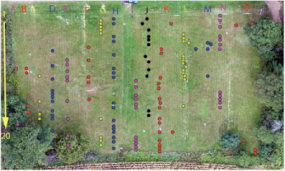
Figure 4 This image was used by the class to assign each feature with an individual alphanumeric code. This code was entered into the “PointID” field of the spreadsheet. 

The photos and drone imagery were uploaded and shared in the class folder on the University’s geography server. The class decided, through discussion, which attributes were to be recorded and how they were to be standardized in the master spreadsheet (see Figure 5a). Every individual entered the attributes for the headstones they had recorded. Problems were encountered when it became apparent that not every headstone visible on the UAV imagery had had attributes recorded, so a second trip was made to the Hadleyville Cemetery by certain benevolent class members to collect the missing data. It became necessary for each student to download the spreadsheet and further edit it to a higher level of organization and accuracy (see Figure5b).

Figure 5a The master spreadsheet was created using google docs so that everyone would have access to it. Having numerous editors making changes simultaneously made for a chaotic time, however, and mistakes were made. 5b These mistakes were remedied to the best of my ability in my own copy of the spreadsheet, which I downloaded and modified further. 

The UAS (drone) imagery was downloaded into ArcMap 10.4.1. Each headstone was digitized as a point feature and saved to a “Graves” feature class. The Point ID was entered as an attribute for each headstone. Photos of the headstones were added into the attribute table as raster fields. ArcMap encountered problems with the process of downloading the photos (see Figure 6) and the final GIS was modified to only include photos that downloaded successfully. A table join was enacted, using the Point ID field, to join the personal modified excel copy of the master spreadsheet to the attribute table of the Graves feature class. 

Figure 6 The error message above was displayed each time a photo was added to the Graves feature class. 

A separate feature class, “Monuments”, was made for the monuments which designated family plots. These were typically large stone markers that had a surname and/or numerous first names inscribed on it but was not being used to mark a specific burial plot. One exception, however, can be seen in the case of N13 which served as the Beardsley family monument (containing details about many family members) and also as the headstone for Clifford Beardsley’s grave. This feature was included in both the Grave and Monument feature classes. 
A third feature class was created to denote the location of the ground control points. 

Results and Discussion

The final GIS map (see Figure 7 for a staionary version supplemented  with locator maps) includes three feature classes; Graves, Monuments, and GCPs. The monument features contain photos that will appear when the user clicks on the monument icon. The interactive version of the final product is available as an ArcMap file. The full attribute table is available here. 

Figure 7 This is a snapshot of the interactive GIS product. Each grave feature includes attribute information about the individual buried  there. The monument features contain photos that will open when clicked on. 

Accuracy would have been increased had a plan for data organization been in place before the data collection began. Possible sources of error include the unstandardized methods of recording attributes on the headstones as a class. Since there was no conferring ahead of time, the data each group recorded was different and each group came up with a separate method for naming the rows and columns to identify the headstone locations. The setup of the cemetery provided a challenge: the headstones were not laid out in a grid or in continuous rows. Initially, multiple headstones were missed and attributes and photos had to be collected later. This would not have been necessary had the collection method been more organized. Also, error and ambiguity about where each stone was located would have been mitigated had the survey-grade GPS worked during data collection.  

Conclusion

Overall, this survey was an excellent learning experience. The class needed to work together to organize data collection with little guidance and few directions beforehand, standardize the disorganized data that was collected in the field, and work together to remedy mistakes. Creativity was required to devise solutions and many lessons were learned.

Unfortunately, the lack of planning and numerous equipment failures also resulted in a mediocre product. The level of accuracy of the data that was collected is questionable, and the amount of attributes that were pushed into categories retroactively means a high probability of mistakes. The photo points intended to go with every grave feature did not work, and the final interactive map is not upload-able to this blog. Still, this GIS product does provide the user with more information about the Hadleyville Cemetery than was previously available, and the attributes it provides are a good place for the township to begin when they make a more thorough record in the future. 

Sources

¹ https://en.wikipedia.org/wiki/Hadleyville,_Wisconsin

² https://en.wikipedia.org/wiki/Hadleyville,_Wisconsin

Field Activity #2 - Data Collection at the Hadleyville Cemetery

Introduction

• Provide background to the problem at hand. What are the problems and challenges facing Hadleyville cemetery?

This field activity was developed in response to a proposal to gather data for production of a detailed and accurate map defining burial plots of a local cemetery.

Deputy Clerk / Treasurer Dale Welke and Clerk / Treasurer Jennifer Meyer of the Town of Pleasant Valley contacted the University of Wisconsin Eau Claire Geography Department to request assistance with mapping the headstones at the Hadleyville Cemetery on County Road HH (Section 04, Twn 25N Range 9W). There is currently no record of the locations of burial plots nor any recorded information about the individuals buried therein. The headstones date back to the 1800’s and several of them are broken, missing, or in bad disrepair due to weathering and erosion.

• Why is the loss of original maps and records a particular challenge for this project?

The lack of recorded information poses a problem on burial plots where the headstone is broken, illegible, or missing. Names, year of death, and birth year will need to be deciphered as best as possible but may not be attainable in every case. Plots with headstones missing are completely unmarked and have the potential to be overlooked. This could lead to the plot being sold again; a situation the Town of Pleasant Valley would like to avoid.

• How will GIS provide a solution to this problem?

Using GIS tools, a map of the Hadleyville Cemetery can be created denoting the location of burial plots. The map will be interactive and will include a digital record of the individual buried there,  whatever information can be deciphered from their headstone. This map can be used by the public as a record of individuals buried in the Hadleyville Cemetery and can also serve the Town of Pleasant Valley by denoting which plots are open and available to be sold.

• What makes this a GIS project, and not a simple map?

The map will be interactive; It will contain embedded photos of each headstone as well as attributes such as the name and sex of individuals, years of birth and death, and the condition/composition of the headstone. 

• What equipment are you going to use to gather the data needed to construct the GIS?

Photos will be taken using an Android mobile device and an EXIFtool script will be used to pull the lat/long coordinates.

A drone provided by the university will be used to map the 1.5 acre cemetery. This data will be the basemap.

• What are the overall objectives of your proposal?

The value added GIS product being proposed is an interactive map of the Hadleyville Cemetery that will include photopoints of each headstone, marked locations of each known burial plot, and information about the individual buried in each plot. 

Methods

• What is the sampling technique you chose to use? Why?

Photopoints were taken using an Android mobile device. These photos, in conjunction with an EXIFtool script, provides GPS coordinates of the headstone in the photo. This sampling technique allowed for ease of access for the surveyors by making use of free downloadable scripts, provided software, and accessible devices.

• What is the accuracy of the equipment you are intending to use? (Be sure to cover each piece of equipment)

Android photo coordinates:

Drone:

• How was the data entered/recorded? Why did you choose this data entry method?

Lat/long coordinates are saved automatically on Android devices when the Location setting is on. Using this data is accurate and simple. 

• How will you transfer the data you gather into a GIS?

Using the EXIFtool, the coordinates will be extracted and can then be downloaded into ArcMap.

• What drawbacks are there to the method you propose? How to the pros outweigh the cons of this method?

This method will work well for legible headstones and headstones that are clearly visible. However, plots with headstones that are missing will be difficult to identify using photopoints, but considering the current lack of information, documentation of the legible headstones is a welcome development.

Conclusion

• How do your methods transfer to the overall objectives of your proposal?

Field Activity #1: Mapping the Hadleyville Cemetery

Introduction

• Provide background to the problem at hand. What are the problems and challenges facing Hadleyville cemetery?

This field activity was developed in response to a proposal to gather data for production of a detailed and accurate map defining burial plots of a local cemetery.

Deputy Clerk / Treasurer Dale Welke and Clerk / Treasurer Jennifer Meyer of the Town of Pleasant Valley contacted the University of Wisconsin Eau Claire Geography Department to request assistance with mapping the headstones at the Hadleyville Cemetery on County Road HH (Section 04, Twn 25N Range 9W). There is currently no record of the locations of burial plots nor any recorded information about the individuals buried therein. The headstones date back to the 1800’s and several of them are broken, missing, or in bad disrepair due to weathering and erosion.

• Why is the loss of original maps and records a particular challenge for this project?

The lack of recorded information poses a problem on burial plots where the headstone is broken, illegible, or missing. Names, year of death, and birth year will need to be deciphered as best as possible but may not be attainable in every case. Plots with headstones missing are completely unmarked and have the potential to be overlooked. This could lead to the plot being sold again; a situation the Town of Pleasant Valley would like to avoid.

• How will GIS provide a solution to this problem?

Using GIS tools, a map of the Hadleyville Cemetery can be created denoting the location of burial plots. The map will be interactive and will include a digital record of the individual buried there,  whatever information can be deciphered from their headstone. This map can be used by the public as a record of individuals buried in the Hadleyville Cemetery and can also serve the Town of Pleasant Valley by denoting which plots are open and available to be sold.

• What makes this a GIS project, and not a simple map?

The map will be interactive; It will contain embedded photos of each headstone as well as attributes such as the name and sex of individuals, years of birth and death, and the condition/composition of the headstone. 

• What equipment are you going to use to gather the data needed to construct the GIS?

Photos will be taken using an Android mobile device and an EXIFtool script will be used to pull the lat/long coordinates.

A drone provided by the university will be used to map the 1.5 acre cemetery. This data will be the basemap.

• What are the overall objectives of your proposal?

The value added GIS product being proposed is an interactive map of the Hadleyville Cemetery that will include photopoints of each headstone, marked locations of each known burial plot, and information about the individual buried in each plot. 

Methods

• What is the sampling technique you chose to use? Why?

Photopoints were taken using an Android mobile device. These photos, in conjunction with an EXIFtool script, provides GPS coordinates of the headstone in the photo. This sampling technique allowed for ease of access for the surveyors by making use of free downloadable scripts, provided software, and accessible devices.

• What is the accuracy of the equipment you are intending to use? (Be sure to cover each piece of equipment)

Android photo coordinates:

Drone:

• How was the data entered/recorded? Why did you choose this data entry method?

Lat/long coordinates are saved automatically on Android devices when the Location setting is on. Using this data is accurate and simple. 

• How will you transfer the data you gather into a GIS?

Using the EXIFtool, the coordinates will be extracted and can then be downloaded into ArcMap.

• What drawbacks are there to the method you propose? How to the pros outweigh the cons of this method?

This method will work well for legible headstones and headstones that are clearly visible. However, plots with headstones that are missing will be difficult to identify using photopoints, but considering the current lack of information, documentation of the legible headstones is a welcome development.

Conclusion

• How do your methods transfer to the overall objectives of your proposal?